About Me
I am a Ph. D. student at Westlake University. I major in Theoretical Physics. My research interest lies in quantum simulation and quantum many-body problem.
Unpublished Research Work
Phase Diagram of Driven-Dissipative Bose-Hubbard Model
The system we study is the driven-dissipative Bose-Hubbard model with two-photon drive, one-photon loss, and two-photon loss. The effective Lindblad master equation is:
\[H = \omega a^+ a + U a^+ a^+ a a + \lambda({a^+}^2+a^2)\] \[\dot{\rho} = \mathcal{L} [\rho] = -i[H,\rho] + \kappa_1 \mathcal{D}[a] + \kappa_2 \mathcal{D}[a^2]\] \[\mathcal{D}[A] = 2A\rho A^+ - A^+ A \rho - \rho A^+ A\]where $\omega$ is the detuning, $U$ is the Kerr non-linearity, $\lambda$ is the two photon drive, $\kappa_{1,2}$ are the one-photon and two-photon loss.
By mean-field analysis and stability analysis, we find two steady state solutions $\alpha_{0,1}$ of the model. The figure plots the region where $|\alpha_0|^2$ is stable (red), $|\alpha_1|^2$ is stable (yellow), and both of them are stable (orange).
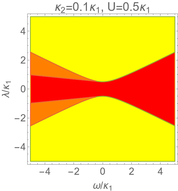
Figure 1. Phase diagram of model
Some interesting things we find about this model:
The steady states we get are:
\[|\alpha_0|^2 = 0\] \[|\alpha_1|^2= \frac{-\kappa_1\kappa_2-\omega U + \sqrt{4\lambda^2(\kappa_2^2 + U^2)-(\kappa_1U-\kappa_2\omega)^2}}{2\kappa_2^2 + 2U^2}\]- If $\kappa_2 = 0$, the boundary of red region on the negative side will become horizontal.
- If $\kappa_1 = 0$, two tips of the yellow region will form a sharp angle and contact.
- If we fix $\lambda$ and control $\omega$, we will see a second-order phase transition on the positive side, and a first-order phase transition on the negative side.
Effects of surface roughness and molecular shapes on gas transport through size-sieving membranes
We study purely repulsive Lennard-Jones particles flowing through pores of membranes piled up with spheres under a pressure gradient, which is maintained by a chemical potential gradient. The gas particles fly from the upstream chamber 1 at chemical potential $\mu_1$ to the downstream chamber 2 at a lower chemical potential $\mu_2$, implemented by the dual control volume grand canonical molecular dynamics (DCV-GCMD) method.
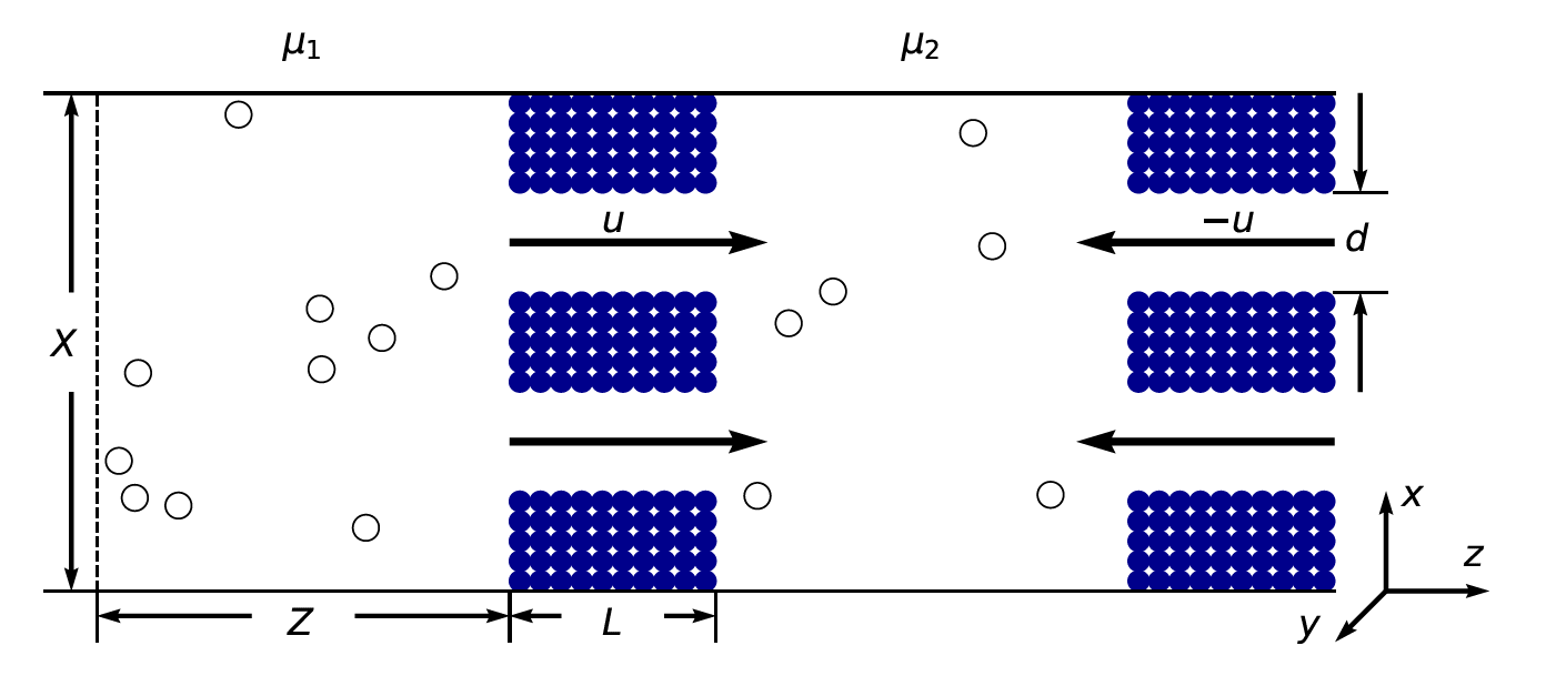
Figure 2. System set up
Real membranes are formed by atoms or molecules with rough surfaces that are different from ideal smooth surfaces. We approach the problem by taking into account the back reflection fraction f (ratio of particles bouncing back) caused by the bumps of rough pores. We apply multiple linear regression and found that:
\[f(\sigma_m,\sigma,n,L) = f_0[1-\exp(-k\frac{L}{\sigma_m})]\exp(-C_1\frac{\sigma}{\sigma_m}-C_2\frac{\sigma^2}{\sigma_m^2}-C_0 n)\]where $f_0$, $C_0$, $C_1$, $C_2$, $k$ are fitting parameters, $\sigma$ is the size of gas particles, $\sigma_m$ is the size of membrane particles, $n$ is the size of pores (number of membrane particles removed along pore diameter), and $L$ is the thickness of the membrane.
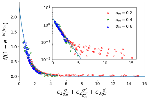
Figure 3. Back fraction function
With the back reflection fraction $f$, we can calculate the diffusivity considering the roughness of membrane $D = D_s (1 − f)$, where $D_s$ means the diffusivity of particles crossing a perfectly smooth membrane. According to hindered diffusion law: $D_s = D_0 (1 − \sigma/d)^2$, where $d$ is pore diamter and the font factor $D_0$ can be estimated by the diffusivity of a point particle entering the circular opening. Then we can get: $D(\sigma/d, n, L) = D_0(1 − \sigma/d)^2 (1 − f)$.
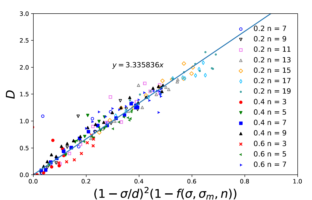
Figure 4. Diffusivity function with back fraction correction